Unit injection exploration

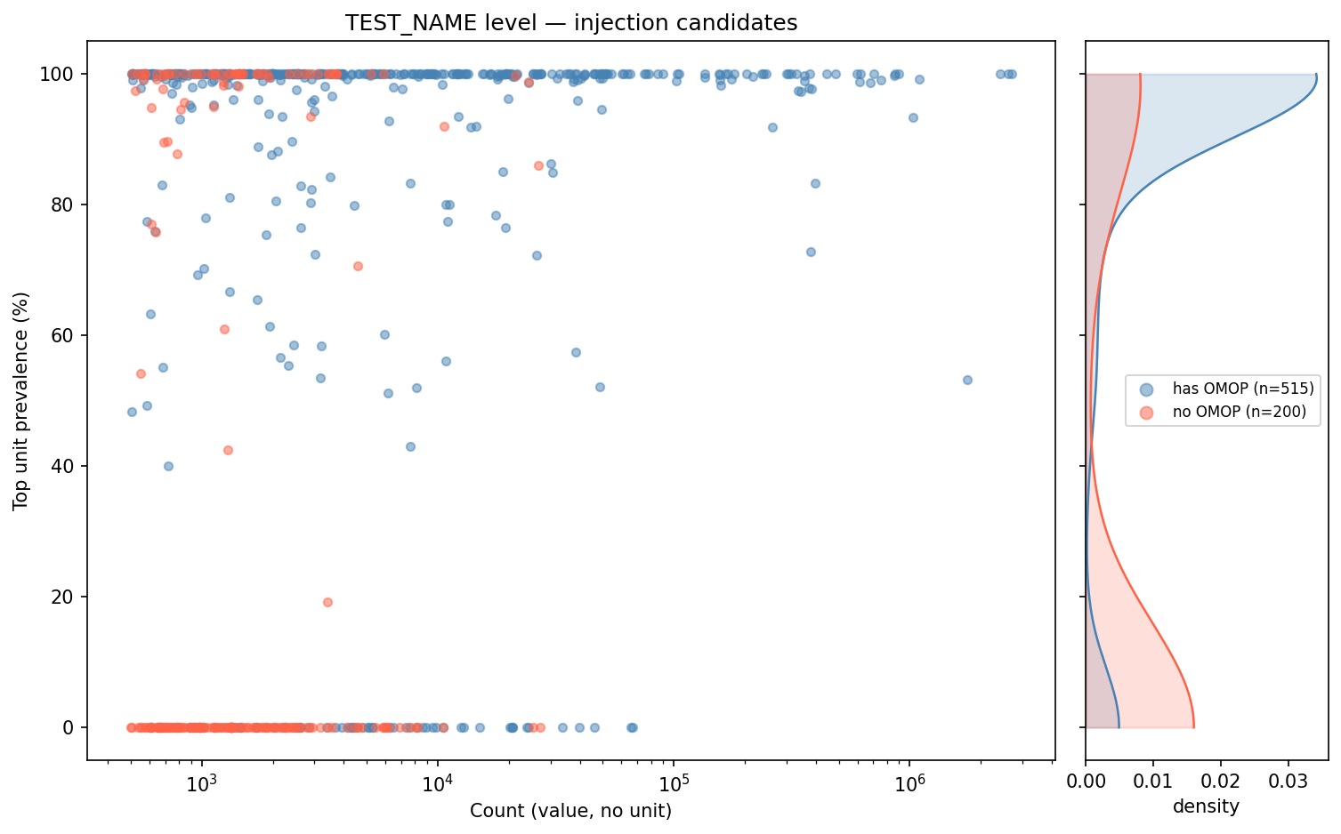
Site: https://finngen.github.io/kanta_lab_preprocessing/injection/

The goal is to identify lab measurements that have a numeric value but are missing a unit, and to characterise the unit distribution of the matching records that do have a unit — so that a unit can be confidently assigned to the missing ones.

Summary

Active threshold: 98% — min count: 500 — 715 TEST_NAMEs, 31,962,504 measurements

Usage

python3 explore_test_name.py <parquet_file> [options]

• <parquet_file>: path to the input parquet file (INJECT.parquet)
• --min-count INT: minimum no-unit records a TEST_NAME must have to be included in plots and injection (default: 1000)
• --prevalence-threshold FLOAT: min dominant-unit prevalence (%) to classify a TEST_NAME as UNAMBIGUOUS (default: 98)
• --min-target-n INT: minimum reference records a unit must have; tests below this are classified NO_DATA (default: 30)
• --dump-dir PATH: cache directory for per-test .npy arrays (default: /mnt/disks/data/kanta/inject/tmp/)
• --omop-unit-table PATH: cache path for the OMOP unit table; built automatically on first run (default: omop_unit_table.tsv)
• --inject: run the injection engine (unambiguous + ambiguous + no_data passes)
• --dip-threshold FLOAT: Hartigan dip test p-value threshold for bimodality (default: 0.05)
• --split-threshold FLOAT: minimum relative KS improvement required to prefer a score-based split over the global fit (default: 0.15)
• --test: small-sample mode — one test per COUNT decile (unambiguous) and top 10 by volume (ambiguous)

Caching behaviour

test_name_counts.tsv and test_name_details.tsv are cached after the first ClickHouse query and reused on subsequent runs — delete them to force a re-query. They are always queried with a fixed baseline of COUNT > 50; --min-count is applied as a post-load filter in Python, so changing it never requires a re-query.

plot_name_level.tsv, test_names_exploration_scatter.png, and summary_table.md are always recomputed from the filtered data.

Per-test .npy arrays are always cached in --dump-dir and reused across runs.

Step 1 — Injection targets (test_name_counts.tsv)

Counts records where at least one value is present (MEASUREMENT_VALUE_EXTRACTED IS NOT NULL OR MEASUREMENT_VALUE_SOURCE IS NOT NULL) but the unit prefix is absent (MEASUREMENT_UNIT_PRE_FIX IS NULL), grouped by TEST_NAME. Cached with COUNT > 50; further filtered to --min-count at runtime.

Columns: TEST_NAME, COUNT

Step 2 — Reference population (test_name_details.tsv)

For every TEST_NAME in Step 1, describes the unit distribution of the records that already have both a value and a unit (MEASUREMENT_VALUE_SOURCE IS NOT NULL AND MEASUREMENT_UNIT_PRE_FIX IS NOT NULL).

Columns: TEST_NAME, COUNT, UNIT, PREVALENCE_DICT

• COUNT: total reference records for this TEST_NAME (across all units)
• UNIT: the most frequent unit
• PREVALENCE_DICT: top-3 units and their percentage share, e.g. {mmol/l:98.5,umol/l:1.5}

Step 3 — Plotting table, scatter plot, and classification

Steps 1 and 2 are merged in Python to produce plot_name_level.tsv, a scatter plot, and a summary table. Each TEST_NAME is assigned a CATEGORY that drives which injection pass it enters.

plot_name_level.tsv

One row per TEST_NAME. Columns include COUNT, N_WITH_UNIT, top_prevalence, CATEGORY, and exploratory CATEGORY_{95,98,99,100} columns.

• COUNT: no-unit record count
• N_WITH_UNIT: total reference records with any unit
• top_prevalence: prevalence (%) of the dominant unit; 0 if no reference records exist

Classification (CATEGORY)

The injection engine only runs tests classified as UNAMBIGUOUS or AMBIGUOUS. NO_DATA tests are written directly to no_data_results.tsv.

OMOP unit table (omop_unit_table.tsv)

Built once from the OMOP LAB mapping files and enriched with per-concept record counts queried from the parquet file. Cached at --omop-unit-table. Each OMOP concept is assigned a CATEGORY:

• SINGLE — only one unit observed in the OMOP data
• EQUIVALENT — multiple units present but all mutually convertible; a CANONICAL_UNIT is available
• MULTIPLE — multiple non-equivalent units; no single canonical unit can be assigned

This table is used to enrich no_data_results.tsv with canonical units.

Two summary tables are written: - summary_table.md — all TEST_NAMEs - omop_summary_table.md — OMOP-mapped subset only

Step 4 — Injection engine (--inject)

With --inject, three passes are run and a coverage check validates that every TEST_NAME in plot_name_level.tsv appears in exactly one output file.

Unambiguous pass → unambiguous_results.tsv

TEST_NAMEs with CATEGORY == UNAMBIGUOUS. The candidate distribution (no-unit records) is compared against the reference distribution for the dominant unit.

One row per TEST_NAME. Columns: TEST_NAME, UNIT, PREVALENCE_DICT, N_CANDIDATE, N_TARGET, CAND_DECILES, TARG_DECILES, KS_STAT, KS_MLOGP, KS_PASS, T_STAT, T_MLOGP, T_PASS, MAD_DIST, MAD_THRESHOLD, MAD_PASS, OUTCOME, NOTES.

Ambiguous pass → ambiguous_results.tsv

TEST_NAMEs with CATEGORY == AMBIGUOUS. Only units with prevalence > 1% and at least --min-target-n reference records are considered.

Pipeline per TEST_NAME:

1. Pre-check: run the full (unsplit) candidate distribution against each qualifying unit.
2. Bimodality check (always runs, even if pre-check passed): test the candidate distribution for bimodality and compute split_improvement — the relative KS gain when the candidate is split at the GMM separator vs. treated globally.
3. Split decision: a split is preferred if split_improvement > --split-threshold AND the two halves favour different best units (same_best_unit == False). If splitting is not preferred and any pre-check passed, the global result is kept.
4. Sub-distribution engine (only if splitting is preferred): the candidate is split into low/high halves at the GMM separator and the engine is re-run on each half × unit.

One row per (TEST_NAME, SUB_DIST) — the best unit only. Best unit selection per sub-distribution:

1. Deciding test quality: PASS_at_KS > PASS_at_T > PASS_at_MAD > FAIL
2. KS statistic ascending (lower = better distributional fit) as tiebreaker within the same quality tier
3. UNIT_PREVALENCE descending as final tiebreaker — prefer the clinically dominant unit when two units are otherwise equivalent

A split_eval_{tag}.png decision-tree figure is saved to --dump-dir for every TEST_NAME.

Columns: TEST_NAME, BIMODAL_STATUS, BIMODAL_SEP, BIMODAL_BC, BIMODAL_DIP_P, BIMODAL_OVERLAP, SCORE_GLOBAL, SCORE_SPLIT, SCORE_IMPROVEMENT, SUB_DIST, UNIT, UNIT_PREVALENCE, PREVALENCE_DICT, N_CANDIDATE, N_TARGET, CAND_DECILES, TARG_DECILES, KS_STAT, KS_MLOGP, KS_PASS, T_STAT, T_MLOGP, T_PASS, MAD_DIST, MAD_THRESHOLD, MAD_PASS, OUTCOME, NOTES.

• SCORE_GLOBAL: best KS statistic achieved across all units on the full candidate distribution (lower = better fit)
• SCORE_SPLIT: size-weighted mean of the best KS statistics for the low and high sub-distributions
• SCORE_IMPROVEMENT: (SCORE_GLOBAL − SCORE_SPLIT) / SCORE_GLOBAL — relative improvement from splitting
• BIMODAL_OVERLAP: GMM overlap coefficient expressed as a percentage. Computed as ∫ min(w₁·f₁(x), w₂·f₂(x)) dx × 100 on a fine grid covering ±4σ from each component mean, where f₁, f₂ are the Gaussian component densities and w₁, w₂ their mixture weights. A value of 0 % means the two modes are perfectly separated; values above ~5–15 % indicate meaningful overlap where values near the separator cannot be confidently assigned to either unit, with direct clinical implications (e.g. a low-mg value mislabelled as g would change the clinical interpretation by orders of magnitude). NA for unambiguous tests and for ambiguous tests where no split was performed.

No-data pass → no_data_results.tsv

TEST_NAMEs with CATEGORY == NO_DATA. No engine is run. The result is enriched with OMOP unit table information; a canonical unit is injected where the OMOP concept has category SINGLE or EQUIVALENT.

Columns: TEST_NAME, COUNT, OMOP_CONCEPT_ID, OMOP_QUANTITY, CATEGORY, N_UNITS, UNITS, CONVERSIONS, OMOP_TOTAL_N, UNIT, PREVALENCE.

• CATEGORY: OMOP unit category (SINGLE, EQUIVALENT, MULTIPLE, or NA)
• UNIT: canonical unit from the OMOP table if available, otherwise blank
• PREVALENCE: fraction of OMOP concept records that are no-unit (COUNT / OMOP_TOTAL_N)

After writing, a breakdown is printed: - no OMOP — TEST_NAMEs with no concept ID - OMOP, unit injected — concept has SINGLE/EQUIVALENT category - OMOP, no unit — concept mapped but MULTIPLE or unknown unit

Unified output → injection_results.tsv

Merge of the unambiguous and ambiguous results with a TYPE column (unambiguous / ambiguous). Does not include no_data rows.

Coverage check

After all three passes, a checksum validates that the union of the three output files equals the full set of TEST_NAMEs in plot_name_level.tsv, with no overlaps and no missing entries. Skipped in --test mode.

Assignment summary

Printed at the end of --inject. Shows, for each category (UNAMBIGUOUS, AMBIGUOUS, NO_DATA) and in total, how many TEST_NAMEs and measurements received a unit (PASS rows), broken out for all TEST_NAMEs and the OMOP-mapped subset.

Injection engine pipeline

Each comparison runs three tests in order. All three always run; the first to decide the outcome wins.

1. KS test — two-sample Kolmogorov–Smirnov. PASS = stat < 0.3 AND p < 0.05. Uses a fast binned approximation (100k bins, Hodges-corrected asymptotic p) above 500k samples; exact scipy otherwise.
2. Welch t-test — fallback if KS fails. PASS = p ≥ 0.05 (means not significantly different).
3. MAD test — last resort. PASS = |median(candidate) − median(target)| ≤ 3 × MAD(target).

Decision rule: KS PASS → PASS. KS FAIL, T PASS → PASS. Both fail → MAD decides. NOTES records the deciding test and how many of the three passed, e.g. PASS_at_T_(2/3).

P-values are stored as −log10(p) throughout (KS_MLOGP, T_MLOGP).

Each comparison produces a 3-panel diagnostic plot saved to --dump-dir: - Panel 1: ECDFs + KS distance marked in red + KS annotation - Panel 2: KDE (linear scale) + dotted mean lines + t-test annotation - Panel 3: KDE (log scale) + MAD band (green = PASS, salmon = FAIL) + median lines + distance arrow

KDE/ECDF rendering downsamples to 50k points. All statistics use the full arrays.

Bimodal check

Before the ambiguous sub-distribution pass, the candidate distribution is tested for bimodality using two statistics:

The candidate array is subsampled to 50,000 points before the dip test and GMM fitting (the dip test is unreliable above ~72k samples and GMM fitting is also faster at this size). All statistics and the separator are computed on this subsample.

Hartigan's dip test (primary gate): p-value < --dip-threshold (default 0.05) declares non-unimodal.

Bimodality coefficient (BC): (skew² + 1) / (excess_kurtosis + 3(n−1)²/((n−2)(n−3))). Values above ~0.555 suggest bimodality.

Both are computed in the space (linear or log) where a 2-component GMM achieves lower BIC. The GMM separator is used to split the candidate distribution.

split_by_score is a separate label assigned when score improvement alone drives the split (SCORE_IMPROVEMENT > --split-threshold and the two halves favour different best units) but the dip test did not find bimodality. When the dip test does confirm bimodality, the bimodal or bimodal_cautious label takes priority even if score improvement is also large — so split_by_score strictly means "split was justified by score despite a unimodal dip result."

The NOTES column in the unified output records the split rationale followed by DIP and OL metrics: - split_by_bimodal at Y | DIP:p,BL:x% — dip-test-confirmed bimodal split at separator Y - split_by_bimodal_cautious at Y | DIP:p,BL:x% — as above, with overlapping modes - split_by_score (+X%) at Y | DIP:p,BL:x% — score-driven split despite unimodal dip result - NO_SPLIT — no split performed (pre-check passed, or unimodal with no score preference)

DIP is the Hartigan dip test p-value; BL is the bimodal overlap percentage (see BIMODAL_OVERLAP above).

BIMODAL_OVERLAP (see above) quantifies how cleanly separated the two modes are after any split. A diagnostic plot (bimodal_{tag}.png) is saved to --dump-dir.